STA 4051 Nonparametric Statistics

Dr. Cohen

Welcome to STA 4051

This course covers an introduction to nonparametric statistics methods as follows:

• Binomial Based Tests
• Rank based Test
• Contingency Tables
• Goodness of fit Test

What is Statistics?

• Statistics deals with 4 subtopics:
  • Data Collection
  • Data Analysis
  • Interpretation of Results
  • Visualization
• Descriptive vs Inferential
• Parametric vs Nonparametric

Nonparamertic Methods?

• Nonparametric methods require few assumptions about the underlying population (e.g. normal)
• Exact p-values for tests and exact coverage probabilities for confidence intervals.
• Nonparametric methods are relatively insensitive to outliers
• Nonparametric methods are only slightly less efficient than their normal theory competitors
• Nonparametric methods apply to data that are nominal, ordinal or ranks
• If a small sample size is used n=3.

Definitions (review)

• Population: is the large body of data that is the target of our interest.
• Sample: is a subset of the population.
• Sample space: is the collection of all possible outcomes of an experiment.
• Event: is any subset of the sample space.

What is Probability? (review)

• Intuitive: A probability is a measure of one’s believe in the occurrence of an event.
• Axiomatic: Consider A is an event in the sample space S then:
  • \(0 \leq P(A) \leq 1\)
  • \(P(S)=1\)
  • The probability of the union of mutually exclusive events is the sum of the probabilities of the individual events.

Random Variables? (review)

• Definition: A function that assigns real numbers to the points in a sample space.
• Discrete: values are finite or countably infinite
• Continuous: values in an interval
• Probability distributions:
  • Discrete: binomial(\(n\),\(p\)), geometric(\(p\)), Poisson(\(\lambda\)), etc.
  • Continuous: N(\(\mu\),\(\sigma^2\)), Gamma(\(\alpha\),\(\beta\)), etc.
  • Sampling distributions: \(\chi^2_{df}\), \(F_{u,v}\), \(t_{n}\)

Expected Values? (review)

Let’s \(X \sim p(x)\) be a discrete r.v., then the expected value:

\[E(X) = \sum_{\forall x} x p(x)\]

Let’s \(X \sim f(x)\) be a continuous r.v., then the expected value:

\[E(X) = \int_{\forall x} x f(x) dx \]

• Variance: \(Var(X) = E(X^2) - E(X)^2\)
• Properties:
  • \(E(a) = a\); \(E(aX+b) = aE(X)+b\)
  • \(Var(a) = 0\); \(V(aX+b) = a^2 Var(X)\)

Introduction to R/RStudio

• R is a free software environment for statistical computing and graphics.

• RStudio is an integrated development environment (IDE) for R and Python, with a console, syntax-highlighting editor, and other features.

• R Markdown provides an authoring framework for data science. You can use a single R Markdown file to both save and execute code to generate high quality reports.

• Quarto is an open-source scientific and technical publishing system.

• In this class, we will use the UWF RStudio Server. Log in using your UWF account. Go to UWF RStudio Server

Quantiles

Definition: The number \(x_p\) (\(0 \leq p \leq 1\)) is called the \(p^{th}\) quantile of a random variable \(X\) if:

• Continuous: \(P(X\leq x_p) = p\)

• Discrete: \(P(X < x_p) \leq p\) AND \(P(X\leq x_p) \geq p\)

We can think of quantiles as points that split the distribution (values of \(X\)) into equal intervals.

Examples:

• 2-quantile \(\equiv\) Median (Q2=\(x_{0.5}\))
• 4-quantile \(\equiv\) quartiles (Q1=\(x_{0.25}\),Q2,Q3=\({0.75}\))
• 100-quantile \(\equiv\) percentile (\(x_{0.01},x_{0.02},\ldots,x_{0.99}\))
• 10-quantiles \(\equiv\) decile (\(x_{0.1},x_{0.2},\ldots,x_{0.9}\))

Quantiles - Example

Let’s \(X\) be a r.v. with PMF:

x	0	1	2	3
P(X=x)	1/4	1/4	1/3	1/6

1. What is \(x_{0.75}\) the upper-quartile?

Solution: Find \(x_{0.75}\) that satisfies \(P(X < x_{0.75}) \leq 0.75\) AND \(P(X\leq x_{0.75}) \geq 0.75\); if more than one value satisfy this then the average of all values is the answer. (\(x_{0.75}\)=2)

2. What is \(x_{0.5}\) the median?

Solution: Find \(x_{0.5}\) that satisfies \(P(X < x_{0.5}) \leq 0.5\) AND \(P(X\leq x_{0.5}) \geq 0.5\); if more than one value satisfy this then the average of all values is the answer.(\(x_{0.5}\)=1.5)

Quantiles - R

Example 1:

x = (1:12) #a vector from 1 to 12
x

 [1]  1  2  3  4  5  6  7  8  9 10 11 12

median= quantile(x,p=c(0.5)) # Median of x
median

50% 
6.5 

quartiles= quantile(x,p=c(0.25,0.5,0.75)) # quartiles of x
quartiles

 25%  50%  75% 
3.75 6.50 9.25 

Example 2:

summary(mtcars$mpg)

   Min. 1st Qu.  Median    Mean 3rd Qu.    Max. 
  10.40   15.43   19.20   20.09   22.80   33.90 

Hypothesis Testing

Hypothesis Testing is the process of inferring from a sample whether or not a given statement about the population appears to be true.

• Null hypothesis - \(H_0\): it is usually formulated for the express purpose of being rejected. No differences. Example: “The process is in-control” in quality control.

• Alternative Hypothesis - \(H_1\): \(H_0\) is rejected. It is the statement that the experimenter would like to prove. There are differences. For example, the alternative hypothesis could be “the quality of the product or service is unsatis- factory” or process is out of control”.

Hypothesis Testing

• The Test Statistic is chosen to be sensitive to the difference between the null hypothesis and the alternative hypothesis.

• Level of significance (\(\alpha\)): When the null hypothesis and the alternative hypothesis have been stated, and when the appropriate statistical test has been selected, the next step is to specify a level of significance \(\alpha\) and a sample size. Since the level of significance goes into the determination of whether \(H_0\) is or is not rejected, the requirement of objectivity demands that \(\alpha\) be set in advance. This is also called Type I Error.

\[ \alpha = P(Reject~H_0~|~ H_0~is~True) \]

Hypothesis Testing

• The Null distribution is the distribution of the test statistic when \(H_0\) is TRUE. This defines the rejection region along with the level of significance.

• The Power: The probability of rejecting \(H_0\) when it is in fact FALSE.

\[Power = 1 - \beta = P(Rejecting~ H_0 | H_0 ~is~FALSE)\]

• P-value is the probability, computed assuming that \(H_0\) is TRUE, that the test statistic would take a value as extreme or more extreme than that actually observed.

• Accepting or Failing to Reject \(H_0\) does not mean that the data prove the null hypothesis to be true. Read the ASA statement on p-values

Binomial Test (Estimation of \(p\))

Binomial distribution

A binomial experiment has the following properties:

• The experiment consists of \(n\) identical independent trials.
• Each trial results in one of two possible outcomes, \(yes\) or \(no\).
• The probability of success (\(yes\)) in each trial is the same, denoted as \(p\).
• The random variable \(Y\) is the number of successes (\(yesS\)) observed during the \(n\) trials.

Binomial Test (Estimation of \(p\))

Binomial distribution

Consider \(Y \sim binom(n,p)\), then \(Y\) can take on values \(0, 1, 2, 3,\ldots, n\). The probability mass function is given by \[\begin{align} p(y)=&P(Y=y)=\binom{n}{y}p^y q^{n-y}, \\ y=&0,1,2,\ldots,n ; \qquad 0\leq p \leq 1 ; \quad q=1-p \end{align}\] The expected value of \(Y\) is: \[\begin{align}E(Y)=np\end{align}\] The Variance \(Y\) is: \[\begin{align} V(Y)=npq \end{align}\]

Binomial Test (Estimation of \(p\))

There are some populations which are conceived as consisting of only two classes:

• member and nonmember,
• married and single,
• male and female.

For such cases all the population observations will fall into either one or the other of the two classes. If we know that the proportion of cases in one class is \(p\), sometimes we are interested to estimate/test the population proportion \(p\).

Binomial Test (Estimation of \(p\))

1.DATA: The sample consists of outcomes of \(n\) independent trails. Each trail has two outcomes (mutually exclusive= they cannot both occur at same time). Let consider \(O_1\) to be \(\#\) of observations in class1 and \(O_2\) to be the \(\#\) of observations in class2. We have \(n=O_1+O_2\).

2.Assumptions: - \(n\) observation are independent. - Each trial has probability \(p\) of resulting in the outcome \(O_1\), where \(p\) is the same for all \(n\) trials.

3.Test Statistic: Since we are interested in the probability of an outcome to be in class1, we will let the test statistic \(T\) be the number of times the outcomes is in class1. Therefore, the test statistic follows the binomial distribution (null distribution) with \(n\) and \(\hat{p}\) (the hypothesized proportion) parameters.

Binomial Test (Estimation of \(p\))

4.Hypothesis: Two-tailed test

\[ H_0: p=p^* \] \[H_1: p \neq p^* \]

• The rejection region is defined by \(t_1\) and \(t_2\) as follows:

\[ P( T \leq t_1) \approx \alpha/2 \] \[ P( T \leq t_2) \approx 1- \alpha/2 \]

• Decision: IF \((T_{Observed} \leq t_1\) OR \(T_{Obs}> t_2\)) then REJECT \(H_0\)

• P-value\(= 2\times \min\{ P( Y \leq T_{Obs}), P(Y \geq T_{Obs}) \}\); If greater than 1 then \(P-value=1\).

Binomial Test (Estimation of \(p\))

4.Hypothesis: Upper-tailed test

\[ H_0: p \leq p^* \]

\[H_1: p > p^* \]

The rejection region is defined by \(t\) as follows:

\[P( T \leq t_2) \approx 1-\alpha \]

• Decision: IF \(T_{Obs} > t\) then REJECT \(H_0\)

• P-value \(=P(Y \geq T_{Obs})\)

Binomial Test (Estimation of \(p\))

4.Hypothesis: Lower-tailed test

\[ H_0: p \geq p^* \]

\[H_1: p < p^* \]

• The rejection region is defined by \(t\) as follows:

\[P( T \leq t_1) \approx \alpha \]

• Decision: IF \(T_{Obs} \leq t\) then REJECT \(H_0\)

• P-value \(=P(Y \leq T_{Obs})\)

Binomial Test - Example

We would like to know whether the passing rate for a course is \(75\%\). We have a sample of \(n=15\) students taking the course and only 8 passed. Level of significance is \(5\%\). Test the appropriate hypothesis as follows:

1. Define the null and alternative hypotheses
   Answer: \[ H_0: p=0.75 \] \[H_1: p \neq 0.75 \]
2. Find the Test statistic observed and null distribution
   Answer: \(T_{obs}=8\) and \(T\sim bin(15,0.75)\)
3. Determine critical values (rejection region)
   Answer: t_1=8 and t_2=14
4. Find P-value
   Answer: p-value=0.1132406
5. Decision and Interpretation
   Answer: Since P-value > 0.05 then Fail to Reject \(H_0\).

Binomial Test - Example

Solution

 binom.test(x = 8, # number of successes (#students pass)
 n = 15, # sample size
 p = 0.75, # hypothesized p
 alternative = 'two.sided', # two-tailed test
 conf.level = 0.95) # Confidence Interval

    Exact binomial test

data:  8 and 15
number of successes = 8, number of trials = 15, p-value = 0.06998
alternative hypothesis: true probability of success is not equal to 0.75
95 percent confidence interval:
 0.2658613 0.7873333
sample estimates:
probability of success 
             0.5333333 

• Interpretation: Fail to Reject \(H_0\). There is evidence to support that the data is compatible with the null hypothesis \(\hat{p}=0.533\); \(95\%CI (0.27,0.79)\).

Sign Test

• The sign test is a binomial test with \(p=0.5\).

• It is useful for testing whether one random variable in a pair \((X, Y)\) tends to be larger than the other random variable in the pair.

• Example: Consider a clinical investigation to assess the effectiveness of a new drug designed to reduce repetitive behavior, we can compare time before and after taking the new drug.

• This test can be use as alternative to the parametric t-paired test.

Sign Test

1.DATA: The data consist of observations on a bivariate random sample \((X_i, Y_i)\), where \(n'\) is the number of the pairs. If the X’s and Y’s are independent, then the more powerful Mann-Whitney test is more appropriate.

Within each pair \((X_i, Y_i)\) a comparison is made and the pair is classified as:

• "+" if \(X_i < Y_i\)
• "-" if \(X_i > Y_i\)
• "0" if \(X_i = Y_i\) (tie)

2.Assumptions: - The bivariate random variables \((X_i, Y_i)\) are mutually independent . - The measurement scale is at least ordinal.

Sign Test

3.Test Statistic: The test statistic is defined as follows:

\[T = \text{Total number of +'s}\]

The null distribution is the binomial distribution with \(p=0.5\) and \(n=\text{the number of non-tied pairs}\).

Sign Test

4.Hypothesis: Two-tailed test

\[ H_0:E(X_i) = E(Y_i) \text{ or } P(+) = P(-) \]

\[H_1: E(X_i) \neq E(Y_i) \text{ or } P(+) \neq P(-) \]

• The rejection region is defined by \(t\) and \(n-t\) where:

\[ P( Y \leq t) \approx \alpha/2 \]

• Decision: IF \((T_{Obs} \leq t\) or $T_{Obs} n-t) $ REJECT \(H_0\)

• P-value\(= 2\times \min\{ P( Y \leq T_{Obs}), P(Y \geq T_{Obs}) \}\)

Sign Test

4.Hypothesis: Upper-tailed test

\[ H_0:E(X_i) \geq E(Y_i) \text{ or } P(+) \leq P(-) \]

\[H_1: E(X_i) < E(Y_i) \text{ or } P(+) > P(-) \]

• The rejection region is defined by \(n-t\) as follows:

\[P( Y \leq t) \approx \alpha \]

• Decision: IF \(T_{Obs} \geq n-t\) REJECT \(H_0\)

• P-value\(= P( Y \geq T_{Obs})\)

Sign Test

4.Hypothesis: Lower-tailed test

\[ H_0:E(X_i) \leq E(Y_i) \text{ or } P(+) \geq P(-) \]

\[H_1: E(X_i) > E(Y_i) \text{ or } P(+) < P(-)\]

• The rejection region is defined by \(t\) where:

\[P( Y \leq t) \approx \alpha \]

• Decision: IF \(T_{Obs} \leq t\) REJECT \(H_0\)

• P-value\(= P( Y \leq T_{Obs})\)

Sign Test - Example

• We are interested in comparing the reaction time before lunch (RTBL) vs the reaction time after lunch (RTAL) using a sample of 18 office workers.
• 12 found their RTBL was shorter
• 1 could not detect a difference

Question: Is the RTAL significantly longer than RTBL?

Solution:

We have \(n'=18\) pairs, each one for a worker:

\[ (RTBL,RTAL) = (X,Y)\]

• "+" if \(RTBL < RTAL\) (12)
• "-" if \(RTBL > RTAL\) (5)
• "0" if \(RTBL = RTAL\) (tie) (1)

then \(n=17\)

Sign Test - Example

Solution

• Define the null and alternative hypotheses

\[ H_0: E(RTBL) \leq E(RTAL) \text{ OR } P(+) \leq P(-) \] \[H_1: E(RTBL) < E(RTAL) \text{ OR } P(+) > P(-) \]

This is an upper-tailed test.

• Test statistic: \(T_{obs}=12\) and \(T\sim bin(17,0.5)\)

• Determine critical values (rejection region): t = 12

• p-value=0.0717316

• Decision: P-value < 0.05 then Reject \(H_0\).

Sign Test - Example R

Solution

 binom.test(x = 12,
 n = 17, 
 p = 0.5,
 alternative = 'g',
 conf.level = 0.95) # Confidence Interval

    Exact binomial test

data:  12 and 17
number of successes = 12, number of trials = 17, p-value = 0.07173
alternative hypothesis: true probability of success is greater than 0.5
95 percent confidence interval:
 0.4780823 1.0000000
sample estimates:
probability of success 
             0.7058824 

• Interpretation: Fail to Reject \(H_0\). There is evidence to support that the data is compatible with the null hypothesis \(\hat{p}=0.71\); \(95\%CI (0.48,1)\).

Tolerance limits

• Confidence limits are limits within which we expect a given population parameter, such as the mean, to lie.
• Tolerance limits are limits within which we expect a stated proportion of the population to lie with a certain probability. Formally:

\[ P(X_{(r)} \leq \text{a fraction q of the population} \leq X_{(n+m-1)}) \geq 1-\alpha \]

Tolerance limits

The tolerance limits can be use to find A sample size \(n\) needed to have at least \(q\) proportion of the population between the tolerance limits with \(1-\alpha\) probability.

\[ n \approx \frac{1}{4} \chi^2_{1-\alpha;2(r+m)} \frac{1+q}{1-q} + \frac{1}{2} (r+m-1)\]

where \(\chi^2_{1-\alpha;2(r+m)}\) is the quantile of a chi-squared random variable.

Tolerance limits

We can find The percent \(q\) of the population that is within the tolerance limits, given n, \(1-\alpha\), \(r\), and \(m\):

\[q=\frac{4n-2(r+m-1)-\chi^2_{1-\alpha;2(r+m)}}{4n-2(r+m-1) + \chi^2_{1-\alpha;2(r+m)}}\]

Tolerance limits - Example

Electric seat adjusters for a luxury car manufacturer wants to know what range of vertical adjustment is needed to be \(90\%\) sure that at least \(80\%\) of population of potential buyers will be able to adjust their seat.

• Range: r=1, m=1
• 1-\(\alpha\) = 0.9
• \(q\) = 0.8

To answer the question we need to find \(n\)

R code

n= 0.25*qchisq(0.9,2*(1+1))*(1+0.8)/(1-0.8) + 0.5*(1+1-1)
n

[1] 18.00374

Next, we need to randomly pick 18 people from the population of potential buyers and collect their adjustments.

R code with tolerance package

#install.packages("tolerance") # install package
library(tolerance)

# How to find Q
distfree.est(n = NULL, # to find sample size
             alpha = 0.1, # 1-alpha is the confidence
             P= 0.8, # fraction of the population 
             side = 2 # two sided interval
               )

Contingency Tables

Definition A contingency table is an array of natural numbers in matrix form where those numbers represent counts / frequencies

	Col 1	Col2	Totals
row 1	a	b	a+b
row 2	c	d	c+d
Totals	a+c	b+d	a+b+c+d

2 x 2 contingency table

Contingency Tables

Chi-squared Test for differences in Probabilities

Data

	Class 1	Class2	Totals
Population 1	a (\(p_1\))	b	\(n_1\) = a+b
Population 2	c (\(p_2\))	d	\(n_2\) = c+d
Totals	\(c_1\) = a+c	\(c_2\)= b+d	N = a+b+c+d

2 x 2 contingency table

Assumption

• Each sample is Random Sample
• The 2 samples are independent
• Each observation can be classified into class 1 and class 2

Contingency Tables

Chi-squared Test for differences in Probabilities

Test Statistic

\[ T= \frac{\sqrt{N} (ad - bc)}{\sqrt{n_1n_2c_1c_1}}\]

Null distirbution: \(T \sim N(0,1)\)

Contingency Tables

Chi-squared Test for differences in Probabilities

Hypothesis: Two-tailed test

\[ H_0:p_1 = p_2 \]

\[H_1: p_1 \neq p_2 \]

• \(p_1\) the probability that a randomly selected obs from the population 1 will be in class 1.

• P-value\(= 2\times \min\{ P( T \leq T_{Obs}), P(T \geq T_{Obs}) \}\)

• Decision: IF p_value < \(\alpha\) then REJECT \(H_0\)

Contingency Tables

Chi-squared Test for differences in Probabilities

Hypothesis: Lower-tailed test

\[ H_0:p_1 = p_2 \]

\[H_1: p_1 < p_2 \]

• \(p_1\) the probability that a randomly selected obs from the population 1 will be in class 1.

• P-value\(= P( T \leq T_{Obs})\)

• Decision: IF p_value < \(\alpha\) then REJECT \(H_0\)

Contingency Tables

Chi-squared Test for differences in Probabilities

Hypothesis: Upper-tailed test

\[ H_0:p_1 = p_2 \]

\[H_1: p_1 > p_2 \]

• \(p_1\) the probability that a randomly selected obs from the population 1 will be in class 1.

• P-value\(= P( T \geq T_{Obs})\)

• Decision: IF p_value < \(\alpha\) then REJECT \(H_0\)

Chi-squared Test - Example 1

The number of items in two car loads.

Data

	Defective	Non defective	Totals
Carload 1	a =13	b=73	\(n_1\) = 86
Carload 2	c = 17	d=57	\(n_2\) = 74
Totals	\(c_1\) = 30	\(c_2\)= 130	N = 160

2 x 2 contingency table

Question: Test whether there are differences in proportions of defective items between the two carloads.

Chi-squared Test - Example 1

1. Define the null and alternative hypotheses
   

\[ H_0: p_1 = p_2 \] \[H_1: p_1 \neq p_2 \]

This is an two-tailed test.

2. Find the Test statistic observed and null distribution
   \(T_{obs}=-1.2695\) and \(T\sim N(0,1)\)

3. Determine critical values (rejection region): +/- 1.96

4. Find P-value: p-value = 0.204

5. Decision: Since P-value > 0.05 then Fail to Reject \(H_0\).

Chi-squared Test - Example 1 with R

data = cbind(c(13,17),c(73,57)) # create data
chisq.test(data, # table data
           correct = FALSE # find p-value without Yates' correction
           ) 

    Pearson's Chi-squared test

data:  data
X-squared = 1.6116, df = 1, p-value = 0.2043

chisq.test(data, # table data
           correct = TRUE # find p-value with Yates' correction
           ) 

    Pearson's Chi-squared test with Yates' continuity correction

data:  data
X-squared = 1.1372, df = 1, p-value = 0.2863

• Interpretation: Fail to Reject \(H_0\). There is evidence to support that the data is compatible with equal proportions \(p-value=0.2\).
• Note: \(T_{obs}^2 = (-1.2695)^2\) = 1.6116303

Chi-squared Test - Example 2

A new toothpaste is tested for men and women preferences.

Data

	Like	Do not like	Totals
Men	a =64	b=36	\(n_1\) = 100
Women	c = 74	d=26	\(n_2\) = 100
Totals	\(c_1\) = 138	\(c_2\)= 62	N = 200

2 x 2 contingency table

Question: Do men and women differ in their preferences regarding the new toothpaste?

Chi-squared Test - Example 2

1. Define the null and alternative hypotheses
   

\[ H_0: p_1 = p_2 \] \[H_1: p_1 \neq p_2 \]

This is an two-tailed test.

2. Find the Test statistic observed and null distribution
   \(T_{obs}=-1.53\) and \(T\sim N(0,1)\)

3. Determine critical values (rejection region): +/- 1.96

4. Find P-value: p-value=0.1260167

5. Decision and Interpretation: Since P-value > 0.05 then Fail to Reject \(H_0\). There is insufficient evidence to support that men and women differ in their preferences regarding the new toothpaste.

Contingency Tables

Fisher’s Exact Test

Data

	col 1	col 2	Totals
row 1	X (\(p_1\))	r-X	r
row 2	c-X (\(p_2\))	N-r-c+X	N-r
Totals	c	N-c	N

2 x 2 contingency table

Assumption

• Each observation can be in one cell
• The row and column totals are fixed.

Contingency Tables

Fisher’s Exact Test

Test Statistic

T = X = number of obs. in row 1 and col 1.

\[ T (H_0) \sim hypergeometric(N,r,C) \]

The PMF is:

\[ P(T=x) = \frac{\binom{r}{x}\binom{N-r}{c-x}}{\binom{N}{c}} \]

x=0,1,2,…,min(r,m)

Contingency Tables

Fisher’s Exact Test

Hypothesis: Two-tailed test

\[ H_0:p_1 = p_2 \]

\[H_1: p_1 \neq p_2 \]

• \(p_1\) the probability that a randomly selected obs from the row 1 will be in col 1.

• P-value\(= 2\times \min\{ P( T \leq T_{Obs}), P(T \geq T_{Obs}) \}\)

• Decision: IF p_value < \(\alpha\) then REJECT \(H_0\)

Contingency Tables

Fisher’s Exact Test

Hypothesis: Lower-tailed test

\[ H_0:p_1 = p_2 \]

\[H_1: p_1 < p_2 \]

• \(p_1\) the probability that a randomly selected obs from the row 1 will be in col 1.

• P-value\(= P( T \leq T_{Obs})\)

• Decision: IF p_value < \(\alpha\) then REJECT \(H_0\)

Contingency Tables

Fisher’s Exact Test

Hypothesis: Upper-tailed test

\[ H_0:p_1 = p_2 \]

\[H_1: p_1 > p_2 \]

• \(p_1\) the probability that a randomly selected obs from the row 1 will be in col 1.

• P-value\(= P( T \geq T_{Obs})\)

• Decision: IF p_value < \(\alpha\) then REJECT \(H_0\)

Fisher’s Exact Test - Example

14 newly hired business majors. - 10 males and 4 females - 2 Jobs are needed: 10 Tellers and 4 Account Rep.

Data

	Account Rep.	Tellers	Totals
Males	X=1	9	r = 10
Females	3	1	4
Totals	c= 4	10	N = 14

2 x 2 contingency table

Question: Test if females are more likely than males to get the account Rep. job.

Fisher’s Exact Test - Example

1. Define the null and alternative hypotheses
   Answer: \[ H_0: p_1 \geq p_2 \] \[H_1: p_1 < p_2 \] This is an lower-tailed test.
2. Find the Test statistic observed and null distribution
   Answer: \(T_{obs}=X=1\) and \(T\sim hypergeometric(14,10,4)\)`
3. Find P-value
   Answer: p-value=0.040959
4. Decision and Interpretation
   Answer: Since P-value < 0.05 then Reject \(H_0\).

Fisher’s Exact Test - Example with R

data = cbind(c(1,3),c(9,1)) # create data
fisher.test(data,alternative = "l")

    Fisher's Exact Test for Count Data

data:  data
p-value = 0.04096
alternative hypothesis: true odds ratio is less than 1
95 percent confidence interval:
 0.000000 0.897734
sample estimates:
odds ratio 
0.05545513 

• Interpretation: Reject \(H_0\). There is evidence to support that the data is compatible with the assumption that females are more likely than males to get the account Rep. job.

The Median Test

Test for equal medians.

\[H_0: \text{All C populations have the same median} \]

\[H_1: \text{At least two populations have different medians} \]

Data

• C random samples are independent
• Arrange the data as follows:
  • Find the Grand Median (GM), that is the median of the combined samples.
  • Set up a 2 by C contingency table as follows:

	Sample 1	Sample 2	…	Sample C	Totals
\(>\) GM	\(O_{11}\)	\(O_{12}\)	…	\(O_{1C}\)	a
\(\leq\) GM	\(O_{21}\)	\(O_{22}\)	…	\(O_{2C}\)	b
Totals	\(n_{1}\)	\(n_{1}\)	…	\(n_{C}\)	N

The Median Test

• Test Statistic

\[ T = \frac{N^2}{ab} \sum_{i=1}^{C} \frac{O^2_{1i}}{n_i} - \frac{Na}{b} \]

Under Null hypothesis: \(T \sim \chi^2_{C-1}\); a chi-square distribution with C-1 degrees of freedom.

• P-value \(=P(T \geq T_{obs})\)

• Decision: IF p_value < \(\alpha\) then REJECT \(H_0\)

The Median Test - Example

• 4 methods of growing corn is used.
• The yield per acre is measured and compared across the 4 methods.

Question: Do the medians yield per acre differ across the 4 methods.

The Median Test - Example

1. Define the null and alternative hypotheses

\[H_0: \text{All methods have the same median yield per acre} \]

\[H_1: \text{At least two of the methods medians differ} \]

2. Set up data: See lecture notes

3. Test statistic:

\[T_{obs} = 17.6\]

Under Null hypothesis: \(T \sim \chi^2_{3}\)

The Median Test - Example R

# install.packages("agricolae")
library(agricolae) # package

data(corn) # data

# The Median Test
median_test_out= Median.test(corn$observation,corn$method)

The Median Test for corn$observation ~ corn$method 

Chi Square = 17.54306   DF = 3   P.Value 0.00054637
Median = 89 

  Median  r Min Max   Q25   Q75
1   91.0  9  83  96 89.00 92.00
2   86.0 10  81  91 83.25 89.75
3   95.0  7  91 101 93.50 98.00
4   80.5  8  77  82 78.75 81.00

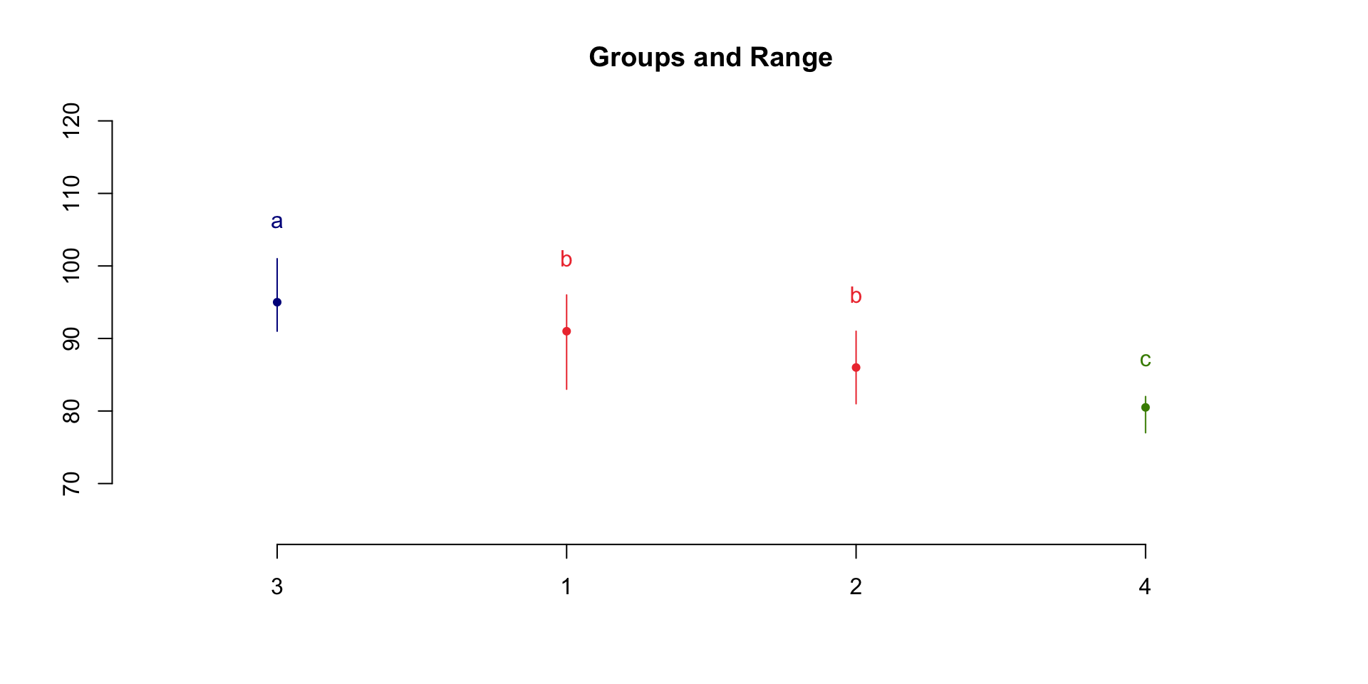
Post Hoc Analysis

Groups according to probability of treatment differences and alpha level.

Treatments with the same letter are not significantly different.

  corn$observation groups
3             95.0      a
1             91.0      b
2             86.0      b
4             80.5      c

The Median Test - Example R

Multiple Comparison

# Visualization
plot(median_test_out)

Goodness-of-Fit Tests - GOF

Test whether a sample is coming from a known distribution. For example, test the normality assumption.

• Kolmogorov-Smirnov Test (KS)
• Shapiro-Wilk Test (SW)
• Chi-squared Test

Goodness-of-Fit Tests - GOF

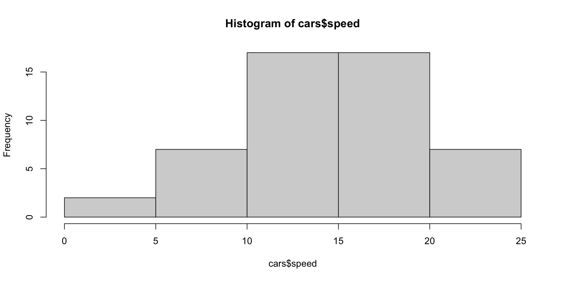
Test if speed data is normally distributed.

Data

hist(cars$speed) # histogram of speed

mean_speed = mean(cars$speed) # mean speed
mean_speed

[1] 15.4

sd_speed = sd(cars$speed) # standard deviation speed
sd_speed

[1] 5.287644

Normality Test

Shapiro Wilk Test

shapiro.test(cars$speed)

    Shapiro-Wilk normality test

data:  cars$speed
W = 0.97765, p-value = 0.4576

Interpretation: Fail to reject H0. There is evidence to support that data is normally distributed.

Kolmogorov Smirnov Test

ks.test(cars$speed,'pnorm',mean_speed,sd_speed)

    Asymptotic one-sample Kolmogorov-Smirnov test

data:  cars$speed
D = 0.068539, p-value = 0.9729
alternative hypothesis: two-sided

Interpretation: Fail to reject H0. There is evidence to support that data is normally distributed.

Normality Test

Chi-squared Test

h = hist(cars$speed,plot = FALSE) # hist of data

Ob = h$counts # observed frequencies in classes
Ob

[1]  2  7 17 17  7

p1 = pnorm(5,mean_speed,sd_speed)# P(X <= 5)
p2 = pnorm(10,mean_speed,sd_speed)-pnorm(5,mean_speed,sd_speed) # P(5<=X <= 10)
p3 = pnorm(15,mean_speed,sd_speed)-pnorm(10,mean_speed,sd_speed) # P(10<=X <= 15)
p4 = pnorm(20,mean_speed,sd_speed)-pnorm(15,mean_speed,sd_speed) # P(15<=X <= 20)
p5 = 1- pnorm(20,mean_speed,sd_speed) # P(X> 20)

Pj = c(p1,p2,p3,p4,p5) # put everything in one array
Pj

[1] 0.02460029 0.12896802 0.31628124 0.33798729 0.19216316

sum(Pj) # should be equal to 1

[1] 1

Ej = Pj*50 # Expected counts
Ej

[1]  1.230015  6.448401 15.814062 16.899365  9.608158

Normality Test

Chi-squared Test

# Chi-squared test for GOF
chisq.test(x=Ob,p = Pj)

    Chi-squared test for given probabilities

data:  Ob
X-squared = 1.3267, df = 4, p-value = 0.8568

The degrees of freedom of the test is df=C-1-k=5-1-2=2. k=2 because we did estimate the mean and variance from the sample. We need to recompute the p-value.

pvalue <- 1-pchisq(1.3267,df=2) # pvalue adjusted for the df
pvalue

[1] 0.5151228

Tests Based on the Ranks

Mann-Whitney Test (Wilcoxon Rank Sum Test)

Comparing two independent samples.

Data

• Two random samples are of interest here. Let \(X_1, X_2, \ldots, X_n\) be a random sample of size \(n\) from population 1. And Let \(Y_1, Y_2, \ldots, Y_m\) be a random sample of size \(m\) from population 2.

• Assign ranks 1 to \(n+m\) to the all observations and let \(R(X_i)\) be the rank assigned to \(X_i\). The same let \(R(Y_i)\) be the rank assigned to \(Y_i\). \(N=n+m\).

• If several samples values are exactly equal to each other (tied), assign to each their average of the ranks that would have been used to them if there had been no ties.

Mann-Whitney Test (Wilcoxon Rank Sum Test)

Assumptions

• Both samples are random samples.
• Mutual independence between the two samples
• At least ordinal

Test Statistic

• If no ties: \(T = \sum_{i=1}^n R(X_i)\)

• If there are ties: \(T_1 = \frac{T - \frac{n(N+1)}{2}}{\sqrt{\frac{nm}{N(N-1)} \sum_{i=1}^N R^2_i -\frac{nm(N+1)^2}{4(N-1)}}}\), where \(\sum_{i=1}^N R^2_i\) is the sum of the squares of all Ranks.

Mann-Whitney Test (Wilcoxon Rank Sum Test)

The null distribution is approximated with the standard normal distribution for \(T_1\). However, \(T\) has the exact distribution for small sample sizes \(<20\).

Hypotheses

Let \(F(x)\) be the distribution function corresponding to \(X\).

Let \(G(x)\) be the distribution function corresponding to \(Y\).

• Two-tailed test

\[ H_0: F(x) = G(x) \quad \text{for all x} \]

\[H_1: F(x) \neq G(x) \quad \text{for some x} \]

The rejection region is defined by the quantiles \(T_{\alpha/2} (T_1)\) and \(T_{1-\alpha/2} (T_1)\). \(\alpha\) is the significance level.

Mann-Whitney Test (Wilcoxon Rank Sum Test)

• Upper-tailed test

\[ H_0: F(x) = G(x)\]

\[H_1: E(X) > E(Y) \]

Here \(X\) tends to be greater than \(Y\).

• Lower-tailed test

\[ H_0: F(x) = G(x)\]

\[H_1: E(X) < E(Y) \]

Here \(X\) tends to be smaller than \(Y\).

Mann-Whitney Test (Wilcoxon Rank Sum Test) - Example R

High temperatures are randomly selected from days in a summer in 2 cities.

Question: Test if the mean high temperature in city1 is higher than the mean high temperature in city2.

temp_city1 = c(83,91,89,89,94,96,91,92,90)
temp_city2 = c(78,82,81,77,79,81,80,81)
wilcox.test(temp_city1,temp_city2,alternative = "g")

    Wilcoxon rank sum test with continuity correction

data:  temp_city1 and temp_city2
W = 72, p-value = 0.0003033
alternative hypothesis: true location shift is greater than 0

Tests Based on the Ranks

Wilcoxon Signed Ranks Test (paired data)

Comparing two dependent samples. This test can be used as an alternative to the paired t-test when the assumptions are not met.

Data

• The data consists of observations on a bivariate random sample \((X_i, Y_i)\), where \(n'\) is the number of the pairs observed. Find the differences \(D_i=Y_i - X_i\). The absolute differences are:

\[ \mid D_i\mid = \mid Y_i - X_i \mid, \qquad i=1,2\ldots,n' \]

• Omit the pairs where the difference is zero. Let \(n\) be the remaining pairs. Ranks from 1 to \(n\) are assigned to the \(n\) pairs according to \(\mid D_i\mid\).

• If several samples values are exactly equal to each other (tied), assign to each their average of the ranks that would have been used to them if there had been no ties.

Wilcoxon Signed Ranks Test (paired data)

Test Statistic

Let \(R_i\) called the signed rank be defined for each pair \((X_i, Y_i)\) as follows: the rank is positive if the D is positive, and negative if the difference D is negative.

• If no ties: \(T^+ = \sum (R_i \text{where} D_i \text{is positive})\). Tables for exact lower quantiles, under \(H_0\), exist. The upper quantile is given: \(w_p = n(n+1)/2 - w_{1-p}\). We will use R.

• If there are ties: \(T = \frac{\sum_{i=1}^n R_i}{\sqrt{\sum_{i=1}^n R_i^2}}\sim\) Standard normal distribution, under \(H_0\).

Wilcoxon Signed Ranks Test (paired data)

Hypotheses

• Two-tailed test

\[ H_0: E(D) = 0 \]

\[H_1: E(D) \neq 0 \]

The rejection region is defined by the quantiles \(T^+_{\alpha/2} (or T)\) and \(T^+_{1-\alpha/2} (or T)\). \(\alpha\) is the significance level.

Wilcoxon Signed Ranks Test (paired data)

• Upper-tailed test

\[ H_0: E(D) \leq 0\]

\[H_1: E(D) > 0 \]

The rejection region is defined by the quantiles \(T^+_{1-\alpha} ( or T)\). \(\alpha\) is the significance level.

• Lower-tailed test

\[ H_0: E(D) \geq 0 \]

\[H_1: E(D) <0 \]

The rejection region is defined by the quantiles \(T^+_{\alpha} (or T)\). \(\alpha\) is the significance level.

Wilcoxon Signed Ranks Test - Example R

• 12 sets of twins
• Measures of the amount of aggressiveness (higher scores mean more aggressive)

Question: Test if first born twin is more aggressive than the other.

first_born= c(86,71,77,68,91,72,77,91,70,71,88,87)
second_born = c(88,77,76,64,96,72,65,90,65,80,81,72)
wilcox.test(first_born,second_born,paired=T,alternative = "g",correct = T,exact = F)

    Wilcoxon signed rank test with continuity correction

data:  first_born and second_born
V = 41.5, p-value = 0.2382
alternative hypothesis: true location shift is greater than 0

P-value > 0.05. Fail to reject H0. There is evidence to suggest that the first born is not more aggressive than the second born.